
How good do you really know the quality of the music you are listening to?
If you have had any sort of trouble in your lifetime trying to recognize how good the final product of an audio file sounds, then you are in the right place. This article will be the first of a small series, deficated to explain what are the factors impacting audio quality in the digital domain. The experts among you might find those explanations oversimplified, however our goal is to put in simple term a complex matter like audio quality and digital audio reproduction. Throughout this first article we will touch the topics of sound analysis, spectral analysis, lossy vs uncompressed or compressed lossless audio.
The toolbox
As any analysis activity, we need to have the right tools, and this is no exception as we’ll be using different softwares to analyze our files. There are many softwares which can help you analyzing your audio files, among the others:
- Audacity, free tool for audio recording, mastering and analysis
- Dynamic Range Meter, a tool to measure DRM of your files
However, my personal favourite is MusicScope, a complete and incredibly advanced toolset to analyze every single detail of your files. I just fell in love with it, since it includes all the measurement you’ll ever want to do to your files, and its so advanced that learning how to exploit its capabilities can be really interesting and instructive. And, we’re extremely happy to have it featured in our shop, as you can buy it here on Volumio, contributing to funding our amazing project.
So, without further talks, may we begin!
Music Sources: Analog vs Digital
In music, there are two types of sources: Analog and Digital. To keep it simple, an analog medium is a way to store sound by physically imprinting the music onto the media, by creating a physical representation on it. That’s why they are called analog: they offer a representation-analogy. Whereas, a digital music source is a digital medium that has digitally encoded a representation of the musical event. This representation is made by a huge amount of 1’s and 0’s lined together, and delivered at a certain speed (clock).
So, while the Analog media are usually a representation of music, digital files are always an approximation, since they are essentially 1 and 0’s tied together by an algorithm. That’s why the quality of a music file is determined by lots of important factors, equally important to define the outcome of the representation. The most obvious is its resolution which is measured in bits and kHz (comparable to megapixel resolution in an image). This topic will be featured in a further article for a more comprehensive dissertation. It might be a better start to examine the qualities of music we want to preserve to get the most “musicality” out of it.
Sound analysis 101: Decibels and Dynamic Range
There are a lot of aspects when it comes to understanding how a song’s final recording achieves it’s worth. Sound level is one of them, measured in decibels or (DB), which is a ratio that uses a logarithm to describe the amount of power, sound pressure, voltage or intensity of the musical piece you are listening to. In order to have virtuous music you want to have an accurate amount and variation of the recorded output.
For a file to be considered with good characteristics then it must have a certain dynamic range level, usually referred as Dynamics. Defining dynamic range is not too complicated as it is the contrast or variation of the quietest and loudest volume that the instrument or musical piece makes. Imagine complete silence and suddenly a drum kicking in: that’s what dynamics in music is all about. Typically, good recordings offer a great output level difference beetween their lowest volume sound and their highest, and that will make you appreciate the artist’s virtuosism.
The problem is that in today’s world of music technology and recordings, the euphonious playback is commonly compressed and limited through dynamic range as it allows for the volume to be louder. Most audio engineers in today’s music industry make the choice to behead dynamics so that their music sounds somewhat louder and easier to listen to when people are sitting in their cars or at social gatherings jamming out to some tunes, and that those music will sound loud even with low quality listening gear.
And that’s a shame since in the process, a very important part of the original music message gets lost, making the music less exciting and vibrant for the discerning listener.
Below is an image that displays the dynamic range of Michael Jackson’s Dangerous trough the years. As you can see, the album’s dynamics have been progressively compressed until getting under the bad side on the DR scale unlike the imprinted and uncompressed files that have a good DR scale. For a detailed and comprehensive explanation, head to the excellent article “It’s the mastering, stupid! ‘How record companies are ruining music” .
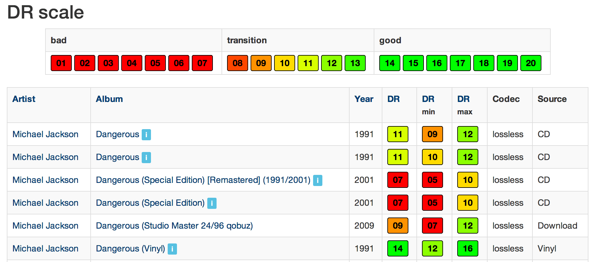
Dynamic Range of MJ’s dangerous across a decade, image from tcervo.com
The understanding of what dynamics are and the range it has plays a key role in the quality of artwork because it displays to the listener what is not only real but also a good sounding audio file. In order for a file to sound good to the ear it must have a good dynamic range and a good dynamic range comes with a balance between a pleasant volume of highs and lows along with the original natural sound.
Long story short: evaluating your file’s dynamic range is a good method to grasp their resemblance with the original event, and the care taken in mastering such musical information. Let’s see how you do it.
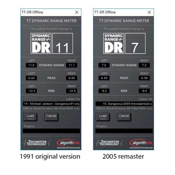
A first method is using Dynamic Range Meter, which will give you a result in form of a number. It ranges from 1 to 20, with values lower than 8 being absolutely bad, values ranging from 8 to 13 begin good but not optimal and values greater than 13 being excellent. Basically, greater the value, greater the Dynamic Range. You can read it in full depth (and compare several measured values) at the Loudness War Info page. So, let’s compare the values of the same song from Michael Jackson, Dangerous, in two different releases (with two different remastering processes). The left one is the original version, with a good (altough not great) DR, while the remaster performs significantly worse.
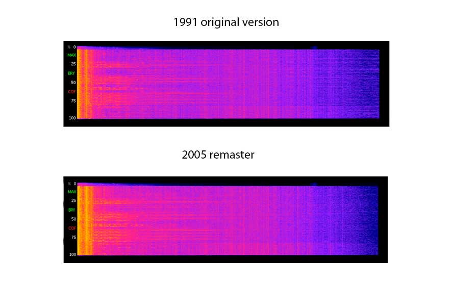
We can have a further insight of what the difference are using MusicScope and its clever Spectral Analysis tool, which we’ll be covering further in the next section. You can visually see the dynamic compression in the second image.
Spectral Analysis
The next step in evaluating how good is your file is to look at the spectral analysis. Basically, it identifies the frequencies of the music file in a visual way: depending on how high or low the notes are the spectral analysis will graph the measurements of “all the frequencies vs. the time” in the file to display them in a spectral diagram. The lower the frequency in the file the lower the notes are and vice versa, the higher the frequency means the higher the notes are. The use of a spectral analysis is a reliable tool to help recognize if the file has been converted from a low quality piece of data to a higher frequency one.
Why is this important? Imagine you want an high resolution image of your favourite panorama. The obvious choice would be taking a picture with an High resolution camera, right? Ok, now imagine that instead you use your high resolution camera to shoot a picture of the same panorama, but instead of focusing the panorama iself you just “scan” a printed picture of it. You will get two equally big files, with lots of information, but only one of them is actually Hi-Res. The same can happen with audio files, with low resolution ones being converted to hi-res.
To tell if a file has been converted from a low quality one to a high frequency one with spectral analysis you want to identify if there are “holes” in the freqency ranges, or if there are frequencies cut-off (musical informations are not stored above or below a certain frequency).
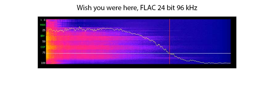
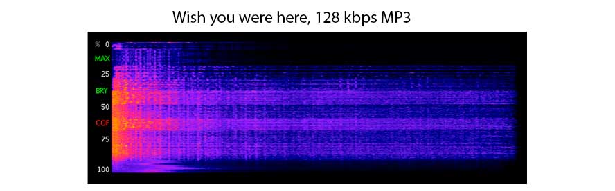
For example, let’s compare the very same track, in this case Wish You were here (from a 24/96 FLAC from master) with different encodings. All measurements are taken with SoundScope’s excelellent Spectrum Analyzer. The below image shows the original file, with all its frequency extension.
Now, we do something funny: we convert this FLAC to 128kbps (CBR, constant bit rate) MP3. Just by looking at it you can understand how much of the original music message has been lost.
And now we do something really weird: we transcode our nasty MP3 back to hi-res FLAC format. At this point you might ask yourself: what’s the point of converting an MP3 back to FLAC? Actually none. But it’s a good way to demonstrate how the starting point of the musical encoding matters so much. Especially when you think on Hi Resolution files that you can buy from specialized websites: they will be actually Hi-Resolution ONLY if they are encoded from the master recording, and not (as sometimes happens) from CD Quality recordings. This practice is called transcoding,
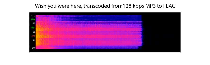
You can clearly see how the transcoding emulates in a linear manner the Spectrals of the low quality MP3. And this is the trick that allows us to spot transcoded files from lower quality.
Lossy vs Compressed Lossless vs Uncompressed Lossless
Now, with a good understanding on what music sources, decibels, and a spectral analysis are and how they work, we can finally move on and get information on the different types of audio formats out there and the role they play in musical entertainment. The formats are either an uncompressed lossless, compressed lossless, or a lossy file.
An uncompressed lossless audio file stores all of the original data, but being uncompressed tends to make the file much larger than other formats. WAV and AIFF files are examples of an uncompressed lossless audio. What you get is all the quality from the original encoding, but a very hefty file.
Compressed lossless files are next on the list and although they store all of the original data too (lossless), they are less larger files due to compressing the musical information without deleting any of the original musical message. For example, by giving silence no bit rates per second they usually have a final result better than an uncompressed lossless file.
Lastly, Lossy formats are always compressed and most of the time they have smaller file sizes than the other formats because they eliminate some of the original information. MP3, AAC, and WMA are all examples of a lossy file. A MP3 file is an encoded format that is used for storage or transmission on digital audio, but it uses compressed lossy data to minimize the size of the file so that the file can still sound like the original uncompressed audio for the person listening.
Long story short: the sweet spot beetween preserving the original quality of the recording without the need to own a datacenter is to prefer compressed lossless, like FLAC (Free Lossless Audio Codec).
That’s all for now, folks. This will be the first article of a series of writings dedicated to understanding, in simple terms, what makes up for a good listening experience in the digital domain. In the next article we’ll be talking about Bitdepth and Frequencies in audio files.
If you feel we did not cover enoug the matter, or you have suggestions for the next topics let us know via comments below, in the meanwhile you can unleash your curiosity and start analyzing your files with the excellent MusicScope Audio Analyzer!